Austin Shijo

As I was preparing for a systems programming competition in C++, I began to relearn CMake, as Cargo had spoilt me too much in the meantime, and I noticed an interesting claim in the tutorial.

Oftentimes the correct answer is to write a tool in a general purpose programming language which solves the problem, and teach CMake how to invoke that tool as part of the build process. Code generation, cryptographic signature utilities, and even ray-tracers have been written in CMake Language, but this is not a recommended practice.

CMake Language Fundamentals

Having written a raytracer earlier, and re-written it for the GPU, this statement caught my eye and made me wonder what would be an even better language to write a raytracer in.

The last re-write involved writing code which had little of a first-principles based approach and mostly depended on a comparatively more complex set of APIs. So I picked the simplest language I knew, BF, because a simple language obviously results in a very simple codebase. In fact, codebases in BF regularly tend to be only a few lines long. Further, Muller’s comment in the README made me want to show a counter example.

The code is available at mTvare6/rayfuck.

Primer

BF is a decidedly simple language, involving only 8 operations and one “data structure”: a one-sided infinite tape of cells, each capable of storing a u8.

On seeing the character >, the data pointer, which points to a cell on the tape, moves rightward, and vice versa on <.

I/O is managed through , and .. The first stores the input byte where the data pointer points and the latter prints it out.

The only primitives other than I/O which allow changing a value are increment and decrement at the data pointer, through + and -.

The limitations should be obvious: there are no n > 1 registers as other machines tend to have, no instruction operating on more than one cell, and no instructions for addition or multiplication.

The last ingredient required to make BF Turing-complete is its loop, written using [ and ]. When the token [ is met, the runtime checks the cell at the data pointer: if it is zero, execution jumps past the matching ], otherwise it enters the loop. At ], it returns to the matching [ if the cell is non-zero and exits the loop otherwise.

A quick exercise would be writing a cat program, try writing one with just 5 characters to get some intuition about the environment.

Premeditation

Having read about it before starting this, I decided to avoid looking up any result or implementation detail and to write down as much as possible from first principles. To keep the scope minimal, and the program an obvious raytracer, I decided to have it render the exact image rendered through the Metal section of RIW.

The C code was a bit too complex regardless, and writing a C parser was clearly out of scope. Writing an unmaintained C parser is something better handled by Anthropic.

I decided that every double [and other datatype like bool] would be represented by combining cells, with half the bits representing the fractional part and the other half representing the integer part, effectively placing a fixed binary point between them. I later got to know that this is called a Q format. Going with the cheaper signed Q8.8 would give a resolution of 1/256 and a range of approximately [-128, 128). But clearly, that wouldn’t be enough, as the sphere used for the ground in the scene had to have r=1000 to appear flat, so I went with the more expensive signed Q16.16 format. It has a resolution of 1/2^16 and a range of [-2^15, 2^15), which is sufficient.

I decided to have the code converted to an SSA-like format [and decided this’ll be the only job for an LLM], where recursive code is made iterative, and variables defined in functions are prefixed in a Hungarian-style notation to avoid name collisions during address lookup for a name.

Similarly, separating the parsing and codegen seemed necessary, dividing complexity into two code regions, with an intermediate “DSL” being used as an IR. The DSL contained simple operations such as abs, add, and, call, copy, div, else, end, eq, func, ge, gt, if, int, le, lt, mul, neg, not, or, print2, print3, set, sqrt, sub, text, var, and while.

The next tricky part was a few library calls. The ones used were sqrt, rand and abs. Initially I planned on using a two-state solution like:

A = (A-B) % 256
B = (B+1) % 256
or
B = (B+A+p) % 256 # for some prime p

but most of these variants have a poor period. I decided to go with the simpler

A = (5*A + 1) % 256

given that it is guaranteed to repeat only after a full sequence of 256 values, which isn’t too bad for this use-case [that is, supersampling anti-aliasing].

sqrt has one obvious candidate, Heron’s formula [of which my memory was refreshed within the same CMake tutorial]. But it was pretty obvious it’d be bad, given it involved division. Repeated subtraction, while producing smaller generated code [which is better, as the interpreter moves less], was still relatively expensive to do. The other candidates were the Taylor series and the “School Method”, which involves long-division.

sqrt(1 + x) = 1 + x/2 - x^2/8
y = 2^16*x
sqrt(2^16 + y) / 2^8  = (1 + y/2^17 - y^2/2^35 )
sqrt(y) / 2^8  = (1 + (y - 2^16)/2^17 - (y - 2^16)^2/2^35 )

Plotting this on Desmos revealed that the fit was poor below an encoded value of 20k, that is, below roughly 0.305, which was a pretty important region. This left me with the long-division method, which was pretty simple. If the real value was x, then the represented value was:

N = x * 2^16

To represent sqrt(x), we need:

N' = sqrt(x) * 2^16
isqrt(N) = sqrt(x) * 2^8
isqrt(2^16 * N) = sqrt(x) * 2^16 = N'

isqrt is justified here, as a difference of one in the encoded result changes the decoded square root by less than 1/2^16, or approximately 0.00001526.

And finally, the whole variable map and corresponding BF addresses would be maintained with a dictionary.

Implementation

With the theoretical bits set up, only clearly simple implementation details were left. Two important primitives were move and copy.

[a, 0]

Move works by continually lowering a value until the cell at the initial data pointer becomes zero, and incrementing the other cell equally every time.

[ # start loop
    - # decrement
    >+ # move right and increment
    < # come back, this cell is used to control the loop
]

as one-liner

[->+<]

And copy works as below, starting with this array:

[a, 0, 0]

using the code.

[->+>+<<]

Turning it into:

[0, a, a]

And now, if needed, the terminal a can be moved inward.

Given that addition, and later division, would involve repeated use of temporary values, which have to be near the value to avoid moving the data pointer around too much, every value in the map also has its temporary-variable slots nearby. These also provide carry cells and other useful scratch space, keeping copies contained.

Multiplication was similarly straightforward, involving multiplying each cell, storing the results and adding them together later. The multiplication step is taken care of through repeated addition. For multiplying two cells, one of them is copied to a temporary place and used as the outer loop, and the other is copied once for every iteration to act as the inner loop. Every iteration of the inner loop increments the result once.

[a, b, a->0, b->0, a + ... + a]

Here a runs out every time and b is decremented when a is zeroed, producing b copies of a.

For the four-cell values, every cell in one is paired with every cell in the other. A multiplication of the cells at i and j is added at i+j in an eight-cell result.

[a0, a1, a2, a3] * [b0, b1, b2, b3]

result[i+j] += a_i*b_j

Since both inputs already had 2^16 in their representation, the lowest 2 cells are discarded when copying back the result.

N_1 = x_1 * 2^16
N_2 = x_2 * 2^16

( N_1 * N_2 ) / 2^16 = N = (x_1 * x_2) * 2^16

Division was slightly less direct but could still be done the way manual long-division is done, by having the dividend be read from its most significant cell and at every step, the old remainder is carried over a cell onto the next.

R = R * 10 + A[next] # school
R = R * 256 + A[next] # here

The divisor then is subtracted from this remainder repeatedly, and one gets added to the result cell. When the remainder becomes negative, the step is reverted and we move to the next cell.

while R >= D:
    R -= D
    result += 1

This requires at most 255 subtractions per cell as we divide across cells and combine them later.

Just as the representation is shifted rightward inflating itself during multiplication, division loses information due to the leftward shift, and some shifting is required in its representation before dividing.

N_1 = x_1 * 2^16
N_2 = x_2 * 2^16

(N_1 / N_2) * 2^16 = (x_1 / x_2) * 2^16 # bits already lost
(N_1 * 2^16) / N_2 = (x_1 / x_2) * 2^16

Throughout these operations, the signs are removed first, and the result is made negative if only one input was negative.

Comparisons share the same smaller operation. Two cells are decremented together until at least one becomes zero, and this continues until there is a difference or the temporary copies are completely zeroed. There was some minor processing involving adding 2^7 to the most significant cell, as otherwise negative numbers technically have a higher value when viewed plainly as bytes.

00 ... 7f  -> positive half
80 ... ff  -> negative half

after adding 128 and wrapping over

80 ... ff  -> positive half
00 ... 7f  -> negative half

Boolean checks involved reading the cells and setting the output to one if any of them was non-zero, to take into account the truthiness tendency of C. The constructed representation had the lowest bit set for true and all bits zero for false. Boolean operations such as and, or and not worked using that bit representation.

Negation uses the -x = ~x + 1 trick. Every cell x is complemented [through 255-x], and then one is added to the lowest cell, carrying over. abs only checks the highest bit of the last cell and performs this negation if it is set.

Given the earlier decision to scope variable names by function and use SSA-style code, functions were extremely straightforward. The codegen notes the function body under its name and emits it inline when call func is seen.

Given loops, if was straightforward.

[- body ]

For an else, another flag starts at one and is cleared by the first body.

And while likewise.

condition
[ 
    body
    move to condition and calculate
]

Artifact

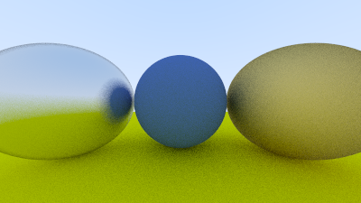
The program was finally 23MB, which is larger than the image itself [which was about 0.9MB], which makes it a rather poor choice for a compression technique.

Using crude calculations, I found that it did 100 ray calculations per minute, that is, one pixel per minute. Given that the image was 400x225, my initial estimate should have been about 62.5 days on my laptop with no further optimizations, but I realized I’d only seen the sky, the bouncing around the spheres would delay the ETA by a lot. So the image above is an approximation of what would be rendered, made using the C code. Of the 1229 [out of 90k] pixels generated at the time of writing, only 10 differ, mostly by a value of one.

Some optimisation is possible. Losing precision to reduce the number of cells touched is the first option if the ground can be approximated worse. The normalization step for random vectors can also be skipped, although that changes the scattering distribution, so it would no longer run the exact bit of code I aimed to reproduce here.